This is a basic Twitter data miner written in Python. It utilizes the Twython, Pandas, Numpy, Matplotlib, Re, Textblob libraries to extract and analyze Twitter data based on a specific search query.
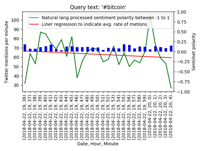
By collecting and organizing the data by chosen time period we are able to visualize the frequency of use of the search term per period as well as assign a positive or negative sentiment to the period based on natural language processing analysis.
We are also able to gain some suggestion as to the rising or falling popularity of the search term by fitting a regression line across the periods, where the slope of the line can suggest an accelerating or decelerating trend.
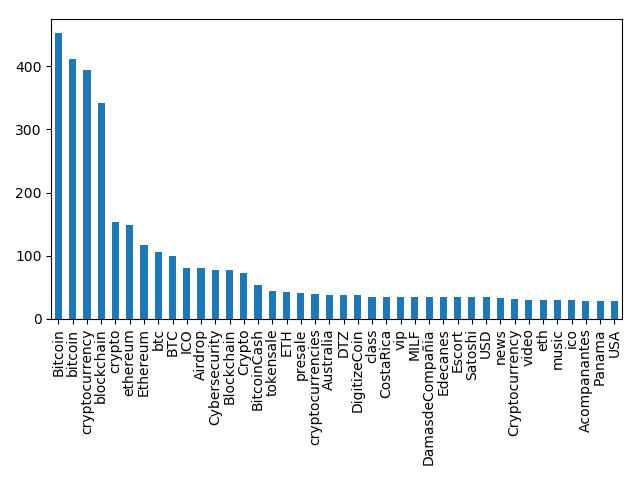
We are also able to aggregate a list of related hashtags that are used along with the search query.
Since this simple data miner utilizes the Twitter standard search API we are limited to 7 days of historic data and completeness is not guaranteed, it is enough for us to build an example that illustrates the possibilities available by mining public opinion through the medium of Twitter.

Let’s proceed then and go over the steps involved in the process.
-
The first thing we need to do is include all the libraries necessary to accomplish our goal.
from twython import Twython
import TwitterApiKeys
import time
import collections
import pandas as pd
import matplotlib.pyplot as plt
import numpy as np
import re
from textblob import TextBlob
-
Step two is to create a file containing our authentication credential for Twitter so we can gain access to API functionality.
consumer_key='YOUR AUTHENTICATION INFO GOES HERE'
consumer_secret='YOUR AUTHENTICATION INFO GOES HERE'
access_token_key='YOUR AUTHENTICATION INFO GOES HERE'
access_token_secret='YOUR AUTHENTICATION INFO GOES HERE'
We are going to obtain authentication keys trough Twitter and place them in TwitterApiKey.py file so that they are separate from our main source file as a good practice since this is information that should not be broadcast publicly.
-
Next we will create a function that collects a number of tweets based on a specific search query.
def MineData(apiobj, query, pagestocollect = 10):

    results = apiobj.search(q=query, include_entities='true',
                             tweet_mode='extended',count='100',
                             result_type='recent')

    data = results['statuses']
    i=0
    ratelimit=1

    while results['statuses'] and i<pagestocollect:

        if ratelimit < 1:
        	#Rate limit time out needs to added here in order to
        	#collect data exceeding available rate-limit
            print(str(ratelimit)+'Rate limit!')
            break

        mid= results['statuses'][len(results['statuses']) -1]['id']-1

        print(mid)
        print('Results returned:'+str(len(results['statuses'])))

        results = apiobj.search(q=query, max_id=str(mid)
                             ,include_entities='true',
                             tweet_mode='extended',count='100',
                             result_type='recent')

        data+=results['statuses']
        i+=1
        ratelimit = int(apiobj.get_lastfunction_header('x-rate-limit-remaining'))

    return data
Some things to note when requesting data with the Twitter search API is that data is returned in an paginated format.
You specify the maximum number of results per page, Twitter will however return any number of results that is under your max number requested per page. The amount of results returned per page is not indicative of the amount of total results left for that search query, so it should not be used as a signal to stop requesting result pages.
To ensure unique search data is contained in each page the max_id parameter needs to be calculate and passed to the API when requesting next page.
Twitter also enforces rate limits on the search requests so this needs to handled appropriately if the data required spans multiple rate limit sessions. The rate limit information and time until rate limit reset is available in JSON header so a sleep period can be easily calculated and implemented, currently the function simply forfeits remaining data if rate limit is exceeded.
-
Now that we have a way to request and gather data lets begin extracting and sorting it ways that can give us the bigger picture. Starting with the associated hashtags.
def ProcessHashtags(data): HashtagData = pd.DataFrame(columns=['HT','ID','Date','RAWDATA_INDEX']) for index,twit in enumerate(data): HashtagData = HashtagData.append(pd.DataFrame({'ID':twit['id'], 'Date':pd.to_datetime(twit['created_at']), 'RAWDATA_INDEX':index, 'HT':[hashtag['text'] for hashtag in twit['entities']['hashtags']]}) , ignore_index=True) return HashtagData -
The tweets time stamp data is next.
def ProcessTimestamp(data): TimestampData = pd.DataFrame(columns=['ID','Date','RAWDATA_INDEX']) for index,twit in enumerate(data): TimestampData = TimestampData.append(pd.DataFrame({'ID':[twit['id']], 'Date':[pd.to_datetime(twit['created_at'])], 'RAWDATA_INDEX':[index]}) , ignore_index=True) return TimestampData -
Finally we run the tweets text through some natural language processing analysis to get the tweets sentiment.
"""
clean_tweet by Rodolfo Ferro
"""
def clean_tweet(tweet):
    '''
    Utility function to clean the text in a tweet by removing
    links and special characters using regex.
    '''
    return ' '.join(re.sub("(@[A-Za-z0-9]+)|([^0-9A-Za-z \t])|(\w+:\/\/\S+)", " ", tweet).split())
Before we can pass the tweet text data to the Textblob library functions for NLP sentiment analysis we must strip all special characters from it, this handy function by Rodolfo Ferro does just that using the regular expressions (Re) library. Thanks Rod.
def ProcessSentiment(data): SentimentData = pd.DataFrame(columns=['ID','Date','Polarity']) for index,twit in enumerate(data): SentimentData = SentimentData.append(pd.DataFrame({'ID':[twit['id']], 'Date':[pd.to_datetime(twit['created_at'])], 'Polarity':[TextBlob(clean_tweet(twit['full_text'])).sentiment.polarity]}) , ignore_index=True) return SentimentData -
With the helper functions finished we can proceed to the actual data mining and analysis. We begin by initializing a Twython object with the our authentication details.
twitter = Twython(TwitterApiKeys.consumer_key, TwitterApiKeys.consumer_secret,
                  TwitterApiKeys.access_token_key,
                  TwitterApiKeys.access_token_secret)
When authenticating with bearer tokens the rate limits are lower as it is designed for twitter applications shared by multiple users, if you want to access the higher application wide rate limits simply authenticate using only the consumer_key and consumer_secret credentials.
-
Next we request and collect tweets based on our chosen search query using the data mine function we created.
dataaccum = MineData(twitter, '#bitcoin',20)
In this case let us search with a query string of #bitcoin since these bits of coins is all I hear the kids talking about.
-
Once we have the actual data we can extract the information we need and sort it appropriately.
#Process Sentiment and group by period giving period sentiment mean value df = ProcessSentiment(dataaccum) SentimentbyDate = df.groupby([df['Date'].dt.date, df['Date'].dt.hour, df['Date'].dt.minute])['Polarity'].mean() #Process Time stamp data and group by period giving number of tweets per period df = ProcessTimestamp(dataaccum) TwittbyDate = df.groupby([df['Date'].dt.date, df['Date'].dt.hour, df['Date'].dt.minute]).size() #Process Hashtags and group by hashtag giving use count across whole data set df = ProcessHashtags(dataaccum) hashtagCountData = df['HT'].value_counts() -
The data is now sorted and split in to periods, we can fit a regression line on to it.
x = np.arange(TwittbyDate.size)

fit = np.polyfit(x, TwittbyDate, 1)
fit_fn = np.poly1d(fit)
-
Finally we plot our processed data in order to visualize it and save it to image files.
#Plot data
TwittbyDate.plot()
plt.plot(x, fit_fn(x), 'r-')
plt.plot(x, TwittbyDate, 'g-', ms=4)
plt.xticks(rotation=90)

plt.xlabel('Date, Hour, Minute')
plt.ylabel('Twitter mentions per minute')
plt.legend(["Natural lang processed sentiment polarity between -1 to 1",
            "Liner regression to indicate avg. rate of metions"])
plt.title("Query text: '#bitcoin'")

ax2=plt.twinx()
ax2.set_ylim(-1,1)

ColorMap = SentimentbyDate > 0
SentimentbyDate.plot.bar(color=ColorMap.map({True: 'b', False: 'r'}),ax=ax2 )

plt.ylabel('Sentimet polarity')
plt.tight_layout()

#Save data plot to image file
plt.savefig('test_graph.png')
Here we set up labels and plot the data on a single x-axis with a twin y-axis for comparison.

hashtagCountData.head(40).plot.bar()
plt.tight_layout()

#Save hashtag data plot to image file
plt.savefig('test_graph_hashtag.png')
And of course we can plot, let us say, top 40 associated hashtags, if of interest.

The use cases here are only limited to our imagination. We could utilize the rate of use data for specific search queries and attempt to find patterns in historic data for when topics catch fire and go viral.
See if a specific regression line slopes across a specific length of time is a predictive factor of viral spread of a topic, or possibly see if that data is better fitted to an exponential function. Once predictive factors are found we can automate the process of looking for topics that might go viral in the hashtags associated with a specific query. Etc etc.
We can take it further by sourcing data from other resources, lets say asset price data or asset trade volumes for example. In such cases we can look for correlation and predictive trends between the data. And indeed my ideas that such approaches are viable were validated in the process of me researching how to implement this Twitter data miner, I ran across a few published papers on the predictive possibilities of Twitter data when it comes to securities.
As big data continues to consolidate and quantify more and more of our behavior online and in real life through the IoT, access to this data becomes more streamlined and computational power grows even further we will see such applications take larger and larger roles in all aspects of society.
Big data, data science and machine learning are indeed only in their infancy.